0. Exploratory Data Analysis (EDA)

Resources:

• ChatGPT
• ClaudeAI
• OpenCV docs
• numpy docs
• matplotlib docs

It would be naïve not to leverage the assimilation of good computer-vision code-practices from a Large Language Model (LLM).

Note that every code block here has been typed out by hand, excepting the Catalogue of Spatial Domain Operators in Section 4 (I let co-pilot autocomplete that block).

Best, Aayush

import cv2
import matplotlib.pyplot as plt

img = cv2.imread("./Castle01.jpg")
plt.imshow(img)
plt.show()
print("Dimensions: ", img.shape)

Dimensions:  (512, 512, 3)

Plotting the other 9 images in a 3x3 subplot.

image_list = [f'Castle{str(i).zfill(2)}.jpg' for i in range(2,11)]
image_list

['Castle02.jpg',
 'Castle03.jpg',
 'Castle04.jpg',
 'Castle05.jpg',
 'Castle06.jpg',
 'Castle07.jpg',
 'Castle08.jpg',
 'Castle09.jpg',
 'Castle10.jpg']

import os

fig, axes = plt.subplots(3,3, figsize=(15,15))
axes = axes.ravel() # unroll axes for indexing ease

image_list = [f'Castle{str(i).zfill(2)}.jpg' for i in range(2,11)]

for i, file in enumerate(image_list):
    img_path = os.path.join('.', file)
    img_sub = cv2.imread(img_path, cv2.IMREAD_GRAYSCALE) # change the grayscales around later

    if img is None:
        print(f"failed to print {file} at {img_path}")
        continue

    axes[i].imshow(img_sub, cmap='gray')
    axes[i].set_title(file)
    axes[i].axis('off')

plt.tight_layout()
plt.show()

Investigating sub-regions

x = 2
y = 1
print(img[1])

[[ 80  80  80]
 [ 61  61  61]
 [ 41  41  41]
 ...
 [108 108 108]
 [129 129 129]
 [169 169 169]]

""" it seems that the dimensionality of the objects should be manipulated to
[ [38, 62, 96, ..., 131, 157, 158],
  [80, 61, 41, ..., 108, 129, 169],
]
"""
img = cv2.imread(os.path.join('.', "Castle01.jpg"), cv2.IMREAD_GRAYSCALE)
print(f"dim: {img.shape}")
print(img[:4])

dim: (512, 512)
[[ 38  62  96 ... 131 157 158]
 [ 80  61  41 ... 108 129 169]
 [ 18  71  73 ... 129  80  79]
 [114  67  98 ... 158 139 132]]

Lambda Function for plotting top_left

top_left = lambda x, y: img[0:y,0:x]
plt.matshow(top_left(300,200), cmap='gray')

<matplotlib.image.AxesImage at 0x15cba6ab0>

Slicing

• note plt.matshow will not work from within a function. it needs an axis to draw on!

img_slice = img[90:160,200:270]
plt.matshow(img_slice, cmap="gray")
plt.show()

Intensities Frequency Histogram

start_max = 0
for i in range(len(img)):
    loop_max = max(img[i])
    if loop_max > start_max:
        start_max = loop_max
print(start_max)

255

import numpy as np

hist = cv2.calcHist([img], [0], None, [256], [0, 256])

plt.figure(figsize=(5,5))
plt.title("intensity frequencies")
plt.xlabel("pixel intensity")
plt.ylabel("frequency")
plt.plot(hist, color='black')
plt.xlim([0,256])
plt.grid(True)
plt.tight_layout()
plt.show()

Last visualisation I promise mum

from mpl_toolkits.mplot3d import Axes3D

x=np.arange(0, img.shape[1])     # note this is backwards in computer vision because x ------> (columns)
y=np.arange(0, img.shape[0])     #                                                   y
X, Y = np.meshgrid(x, y)         #                                                   |
fig = plt.figure(figsize=(10,8)) #                                                   |
ax = fig.add_subplot(111, projection='3d') #                                         |
ax.plot_surface(X, Y, img, cmap='gray', edgecolor='none') #                           v
ax.set_title('z axis is intensity, xy plane coords') #                               = (rows)
ax.set_xlabel('x')
ax.set_ylabel('y')
ax.set_zlabel('z')
plt.tight_layout()
plt.show()

holy crap, check out the top angle!

it looks exactly like the original image!

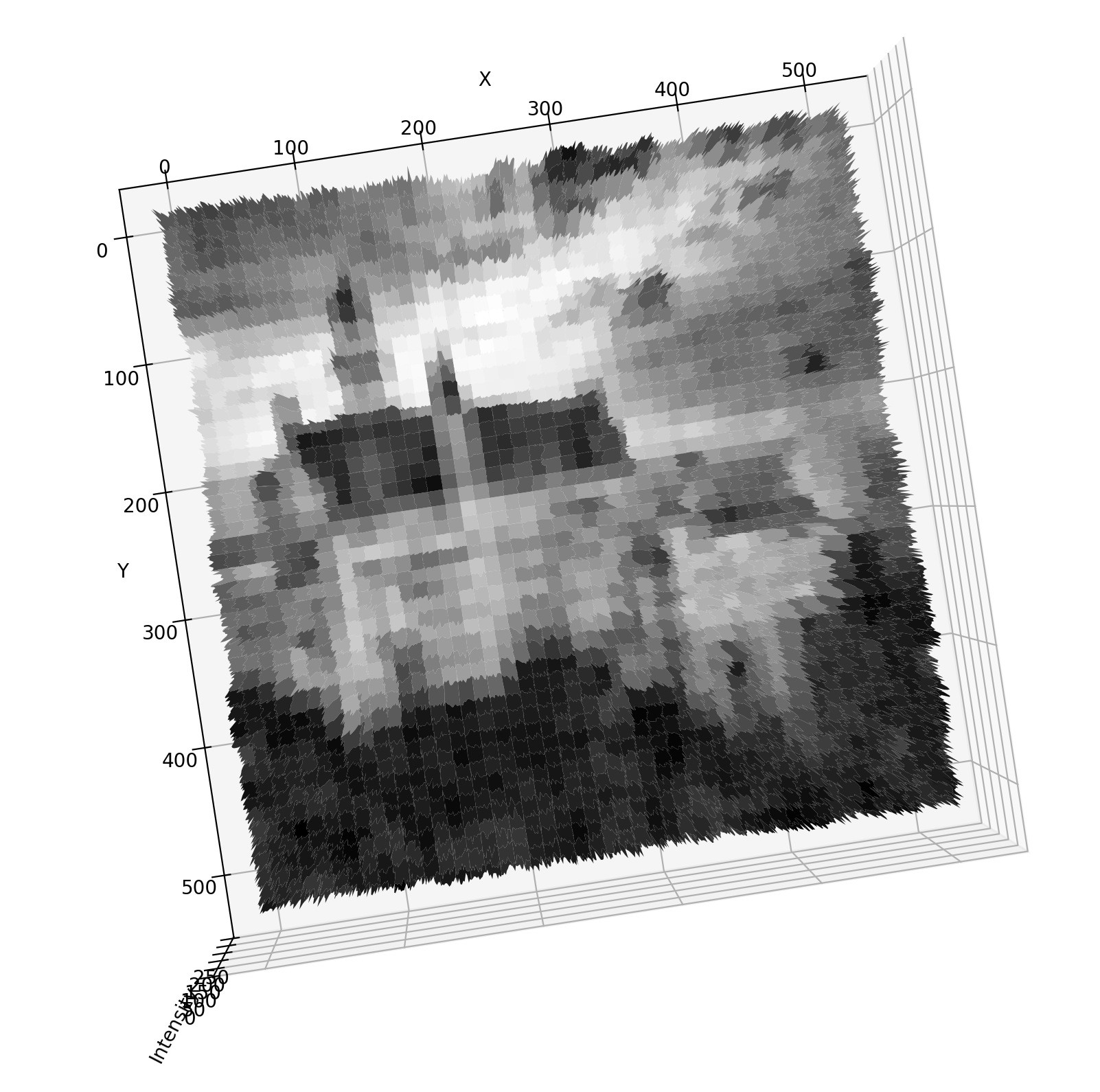
(note to marker: if at this point you cannot realise that this is almost entirely my own work you might be damaged. c.f. abaj.ai for intellectual evidence of the mastery of this content.)

1. Averaging

todo:

• calculate average of 10 images
• how much noise reduction is theoretically possible? (what factor should the std dev of the noise drop?)
• how much noise reduction was actually accomplished?
  • measure std dev in white part of sky for averaged and noisy images. compare them.

intensity thresholding (for fun)

ret,thresh1 = cv2.threshold(img,155,255,cv2.THRESH_BINARY)
ret,thresh2 = cv2.threshold(img,127,255,cv2.THRESH_BINARY_INV)
ret,thresh3 = cv2.threshold(img,127,255,cv2.THRESH_TRUNC)
ret,thresh4 = cv2.threshold(img,127,255,cv2.THRESH_TOZERO)
ret,thresh5 = cv2.threshold(img,127,255,cv2.THRESH_TOZERO_INV)
 
titles = ['Original Image','BINARY','BINARY_INV','TRUNC','TOZERO','TOZERO_INV']
images = [img, thresh1, thresh2, thresh3, thresh4, thresh5]
 
for i in range(6):
    plt.subplot(2,3,i+1),plt.imshow(images[i],'gray',vmin=0,vmax=255)
    plt.title(titles[i])
    plt.xticks([]),plt.yticks([])
 
plt.show()

averaging subplots (the actual task 😅)

image_list_all = [f'Castle{str(i).zfill(2)}.jpg' for i in range(1,11)]
images = []
for file in image_list_all:
    img_i = cv2.imread(os.path.join('.', file), cv2.IMREAD_GRAYSCALE)
    if img is None:
        print(f"failed to load {img_i}")
    else:
        images.append(img_i.astype(np.float32)) # using np floats for averaging.

N_values = [2, 4, 6, 8, 10]

fig, axes = plt.subplots(1, 5, figsize=(20,5))
for ax, N in zip(axes, N_values):
    avg_img = np.mean(images[:N], axis=0) # average first N images, where we index on N
    avg_img = np.clip(avg_img, 0, 255).astype(np.uint8) # convert back for plotting

    ax.imshow(avg_img, cmap='gray')
    ax.set_title(f'N = {N}')
    ax.axis('off')

plt.tight_layout()
plt.show()

Theoretical Noise Reduction

We know that standard deviation is equal to $\sigma$, and that our original image has variance composed of the i.i.d errors $n_i$:

\begin{align} \text{VAR}\left[\frac{1}{N}\sum_{i=1}^{N} n_i(x,y)\right] &= \frac{\sigma^2(x,y)}{N}\\ \Rightarrow \text{STD} &= \frac{\sigma(x,y)}{\sqrt{N}} \end{align}

Thus, theoretically we are able to achieve noise reduction by a factor of $$\frac{1}{\sqrt{N}}$$

(note to marker: I am taking MATH3611 and MATH2901 at the moment; this mathematics is trivial to me.)

Empirical Noise Reduction

we are going to use the below rectangle of sky for measurements!

img = cv2.imread("./CastleAveraged.jpg", cv2.IMREAD_GRAYSCALE) # just to make sure.
print(img.shape)
# slice co-ords.
top, bottom = 130, 160
left, right = 200, 230
width = right - left
height = bottom - top

fig, ax = plt.subplots()
ax.imshow(img)

rect = plt.Rectangle((left, top), width, height,
                     linewidth=2, edgecolor='red', facecolor='none')
ax.add_patch(rect)

plt.axis('off')
plt.imshow(img, cmap='gray') # import cmap!
plt.show()

(512, 512)

measuring std

img_slice = img[130:160,200:230] # [y_start: y_end, x_start: x_end]
plt.matshow(img_slice, cmap="gray")
plt.show() # of this patch of sky:

x, y, w, h = 200, 130, 30, 30
std_orig = np.std(images[0][y:y+h, x:x+w])

avg_img = np.mean(images[:10], axis=0)
std_avg = np.std(avg_img[y:y+h, x:x+w])

theoretical = std_noisy / np.sqrt(N)
actual = std_avg
ratio = actual / theoretical

print(f"Results:")
label_width = 23
print(f"\t{'Theoretical STD':<{label_width}} = {theoretical:.2f}")
print(f"\t{'Actual STD':<{label_width}} = {actual:.2f}")
print(f"\t{'Ratio (actual / theory)':<{label_width}} = {ratio:.2f}")

Results:
	Theoretical STD         = 11.35
	Actual STD              = 6.67
	Ratio (actual / theory) = 0.59

bonus marks, for N = 2, 4, 6, 8:

import pandas as pd

results = []

for N in [2, 4, 6, 8, 10]:
    avg_img = np.mean(images[:N], axis=0)
    std_avg = np.std(avg_img[y:y+h, x:x+w])
    
    theoretical = std_noisy / np.sqrt(N)
    actual = std_avg
    ratio = actual / theoretical

    results.append({
        'N': N,
        'Theoretical STD': theoretical,
        'Actual STD': actual,
        'Ratio': ratio
    })

df = pd.DataFrame(results)
print(df)

    N  Theoretical STD  Actual STD     Ratio
0   2        25.374027   13.246527  0.522051
1   4        17.942146    9.642165  0.537403
2   6        14.649701    8.121696  0.554393
3   8        12.687013    7.222329  0.569269
4  10        11.347610    6.668942  0.587696

discussion

we obtained an empirical standard deviation reduction of about $1/2$.

saving the averaged file

image_list_all = [f'Castle{str(i).zfill(2)}.jpg' for i in range(1,11)]
images = []
for file in image_list_all:
    img_i = cv2.imread(os.path.join('.', file), cv2.IMREAD_GRAYSCALE)
    if img is None:
        print(f"failed to load {img_i}")
    else:
        images.append(img_i.astype(np.float32)) # using np floats for averaging.

N = 10
avg_img = np.mean(images[:N], axis=0) # average first N images, where we index on N
#avg_img = np.clip(avg_img, 0, 255).astype(np.uint8) # convert back for plotting
print(avg_img)
print(avg_img.shape)
print(type(avg_img))
print(avg_img.dtype)
#cv2.imwrite('CastleAveraged.jpg', avg_img) # NEWSFLASH: JPG does not store bigger than UINT8 !!!
#cv2.imwrite('CastleAveraged.png', avg_img) # this doesn't work either :(
np.save('CastleAveraged.npy', avg_img)  # saves as float32 (or whatever dtype)

[[ 75.9  81.4  61.8 ... 127.2 115.2 119.7]
 [ 80.   75.   61.7 ... 115.3 117.1 130.6]
 [ 67.8  87.4  87.8 ... 118.  120.8  99.7]
 ...
 [ 46.6  55.3  84.6 ...  51.9  57.8  47.5]
 [ 67.6  64.   56.7 ...  43.7  45.6  66.8]
 [ 53.6  43.8  42.3 ...  35.   52.1  50.8]]
(512, 512)
<class 'numpy.ndarray'>
float32

2. DoG

todo: - given the averaged image, convolve the difference of f with h1 and h2.

loading avg img

#####
# loading from CastleAveraged.npy:
avg_img = np.load('CastleAveraged.npy')
print(avg_img)
avg_img.shape
avg_img.dtype

[[ 75.9  81.4  61.8 ... 127.2 115.2 119.7]
 [ 80.   75.   61.7 ... 115.3 117.1 130.6]
 [ 67.8  87.4  87.8 ... 118.  120.8  99.7]
 ...
 [ 46.6  55.3  84.6 ...  51.9  57.8  47.5]
 [ 67.6  64.   56.7 ...  43.7  45.6  66.8]
 [ 53.6  43.8  42.3 ...  35.   52.1  50.8]]

dtype('float32')

convolving f with h1 and h2 in subplot

unnorm_h1 = np.array([
    [0,0,0,0,0],
    [0,1,2,1,0],
    [0,2,4,2,0],
    [0,1,2,1,0],
    [0,0,0,0,0]
], dtype=np.float32)

unnorm_h2 = np.array([
    [1,4,6,4,1],
    [4,16,24,16,4],
    [6,24,36,24,6],
    [4,16,24,16,4],
    [1,4,6,4,1]
], dtype=np.float32)

h1 = unnorm_h1 / unnorm_h1.sum()  # divide by 16
h2 = unnorm_h2 / unnorm_h2.sum()  # divide by 256

conv_h1 = cv2.filter2D(avg_img, -1, h1)
conv_h2 = cv2.filter2D(avg_img, -1, h2)

fig, axes = plt.subplots(1, 2, figsize=(10,5))
axes[0].imshow(conv_h1, cmap='gray')
axes[0].set_title('f * h1')
axes[1].imshow(conv_h2, cmap='gray')
axes[1].set_title('f * h2')
#for ax in axes:
#    ax.axis('off')
plt.tight_layout()
plt.show()

okay applying the DoG

img_float = img.astype(np.float32)

# Filter using float32 precision
conv_h1 = cv2.filter2D(img_float, -1, h1)
conv_h2 = cv2.filter2D(img_float, -1, h2)

# convolution of the difference (FAST)
dog_kernel = h1 - h2
conv_dog_1 = cv2.filter2D(img_float, -1, dog_kernel)

# difference of the convolutions (SLOW)
conv_dog_2 = conv_h1 - conv_h2

# Check max absolute difference
np.max(np.abs(conv_dog_1 - conv_dog_2))  # should be ~0

np.float32(0.0)

fig, axes = plt.subplots(1, 3, figsize=(15,5))
axes[0].imshow(conv_dog_1, cmap='gray')
axes[0].set_title('f * (h1 - h2)')
axes[1].imshow(conv_dog_2, cmap='gray')
axes[1].set_title('f * h1 - f * h2')
axes[2].imshow(np.abs(conv_dog_1 - conv_dog_2), cmap='gray')
axes[2].set_title('Difference (assert 0)')
for ax in axes:
    ax.axis('off')
plt.tight_layout()
plt.show()

analysis

the computation difference exists because doing 1 convolution is cheaper than 2 convolutions (why?).

the distributivity of the convolution guarantees the results are the same.

saving the fast conv

np.save('CastleDoG.npy', conv_dog_1)  # saves as float32 (or whatever dtype)
cv2.imwrite('CastleDoG.jpg', conv_dog_1)

True

3. Discrete FFT

seems simple enough:

• compute the magnitude of 2d transform for averaging
• do same for dog
• explain the difference

loading data

dog_img = np.load('CastleDoG.npy')
print(dog_img)
dog_img.shape
plt.imshow(dog_img, cmap='gray')
plt.axis('off')
plt.show()

[[ 1.4375     -1.1953125  -3.734375   ...  0.8125      0.859375
   1.125     ]
 [ 0.5234375  -0.453125   -1.453125   ... -0.21875    -0.48046875
  -0.359375  ]
 [-1.0234375  -0.0078125   0.875      ... -0.3671875  -1.4023438
  -2.2109375 ]
 ...
 [ 0.6875      1.5625      4.2773438  ...  0.640625    1.3945312
   1.515625  ]
 [ 0.015625   -0.38671875  0.34375    ... -0.34765625  2.265625
   2.921875  ]
 [ 0.140625   -2.7109375  -5.109375   ... -2.5         0.8984375
   2.25      ]]

avg_img = np.load('CastleAveraged.npy')
print(avg_img)
avg_img.shape
plt.imshow(avg_img, cmap='gray')
plt.axis('off')
plt.show()

[[ 75.9  81.4  61.8 ... 127.2 115.2 119.7]
 [ 80.   75.   61.7 ... 115.3 117.1 130.6]
 [ 67.8  87.4  87.8 ... 118.  120.8  99.7]
 ...
 [ 46.6  55.3  84.6 ...  51.9  57.8  47.5]
 [ 67.6  64.   56.7 ...  43.7  45.6  66.8]
 [ 53.6  43.8  42.3 ...  35.   52.1  50.8]]

## applying transforms
print(avg_img - dog_img)

[[ 74.4625    82.595314  65.53438  ... 126.3875   114.34062  118.575   ]
 [ 79.47656   75.453125  63.153126 ... 115.51875  117.58047  130.95938 ]
 [ 68.82344   87.407814  86.925    ... 118.36719  122.20235  101.910934]
 ...
 [ 45.9125    53.7375    80.322655 ...  51.259377  56.405468  45.984375]
 [ 67.58437   64.38672   56.35625  ...  44.047657  43.334373  63.878128]
 [ 53.459373  46.510937  47.409374 ...  37.5       51.20156   48.55    ]]

import numpy as np
import matplotlib.pyplot as plt

img_float = avg_img
def show_dft(image, title="DFT Magnitude Spectrum"):

    f = np.fft.fft2(image)
    
    # shift zero-frequency to center
    fshift = np.fft.fftshift(f)
    
    # compute magnitude spectrum
    magnitude_spectrum = np.abs(fshift)
    
    # use log scale for visibility
    magnitude_spectrum_log = np.log1p(magnitude_spectrum)

    plt.figure(figsize=(6,6))
    plt.imshow(magnitude_spectrum_log, cmap='gray')
    plt.title(title)
    plt.axis('off')
    plt.savefig(f"{title}.jpg")
    plt.show()
    
    return fshift, magnitude_spectrum_log

_ = show_dft(img_float, title="DFT of Averaged Image")
_ = show_dft(conv_dog_1, title="DFT of DoG Image")

Discussion

Here is what the 2 images look like:

Part 1: DFT of Averaged Image

Part 2: DFT of DoG Image

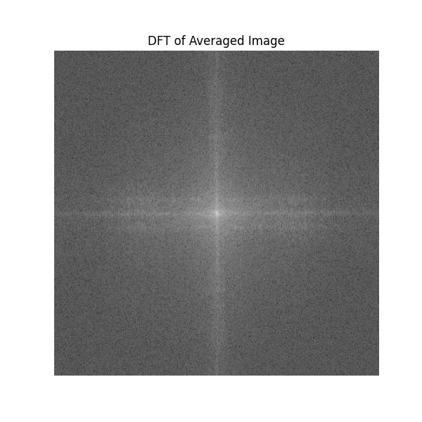
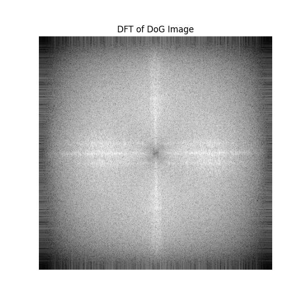
Image 1: Part 1:

Recall that our aim was to reduce the high-frequency noises from the images by a factor of $1/\sqrt{n}$. We did this by applying a low-pass filter in the frequency domain.

Inspecting the first image (on the left above), we have an image the demonstrates "centering" of the low frequencies, and a "darkening effect" as we move outwards. This represents an increase in the dulling of the high-frequency edges / noises.

Image 2: Part 2:

The result of applying the Difference of Gaussians (DoG) (which turns out to be a "bandpass edge detector"):

• Central Dipl there’s a dark spot in the middle => low frequencies are suppressed, which is what DoG does — it removes slow-varying regions.
• Mid-to-High Frequencies Boosted: the image is much brighter overall, especially in the radial band surrounding the center. This shows enhancement of edges and fine details.

Ultimately, what the DoG filter has accomplished is that areas where the image changes abruptly are emphasised. These areas are (naturally) edges and smaller details.

This table is an effect summary of our work in this Notebook

	Averaged Image	DoG Image
Low Frequencies	Strong	Suppressed
High Frequencies	Weak (denoised)	Boosted (edges/textures)
Center of DFT	Bright	Dark
Visual Goal	Smooth, clean	Highlights structure

avg_img = np.load('./CastleAveraged.npy')

4. Extra Spatial Domain Operations

I was curious as to what it would take to implement the rest of the transformations that Erik was ranting about in the lectures.

They all actually turn out to be very simple to implement once you learn the opencv syntax!

# (note-to-marker: I can implement MLP from scrach in Pytorch; this to me is nothing but a change of syntax.)

# contrast stretching
def contrast_stretching(image, low_in, high_in, low_out=0, high_out=255):
    """
    Perform contrast stretching on the input image.
    
    Parameters:
    - image: Input image (numpy array).
    - low_in: Lower bound of input intensity range.
    - high_in: Upper bound of input intensity range.
    - low_out: Lower bound of output intensity range (default 0).
    - high_out: Upper bound of output intensity range (default 255).
    
    Returns:
    - Stretched image (numpy array).
    """
    stretched = np.clip((image - low_in) * (high_out - low_out) / (high_in - low_in) + low_out, low_out, high_out)
    return stretched.astype(np.uint8)
# Example usage
img_contrast_stretched = contrast_stretching(avg_img, low_in=50, high_in=200)
plt.imshow(img_contrast_stretched, cmap='gray')
plt.axis('off')
plt.title("Contrast Stretched Image")
plt.show()
# histogram equalization
def histogram_equalization(image):
    """
    Perform histogram equalization on the input image.
    
    Parameters:
    - image: Input image (numpy array).
    
    Returns:
    - Equalized image (numpy array).
    """
    hist, bins = np.histogram(image.flatten(), 256, [0, 256])
    cdf = hist.cumsum()  # cumulative distribution function
    cdf_normalized = cdf * 255 / cdf[-1]  # normalize to [0, 255]
    
    equalized_image = np.interp(image.flatten(), bins[:-1], cdf_normalized)
    return equalized_image.reshape(image.shape).astype(np.uint8)
# Example usage
img_hist_eq = histogram_equalization(avg_img)
plt.imshow(img_hist_eq, cmap='gray')
plt.axis('off')
plt.title("Histogram Equalized Image")
plt.show()
# Gaussian smoothing
def gaussian_smoothing(image, kernel_size=5, sigma=1.0):
    """
    Perform Gaussian smoothing on the input image.
    
    Parameters:
    - image: Input image (numpy array).
    - kernel_size: Size of the Gaussian kernel (default 5).
    - sigma: Standard deviation of the Gaussian (default 1.0).
    
    Returns:
    - Smoothed image (numpy array).
    """
    # Ensure image is float32 for OpenCV compatibility
    image = image.astype(np.float32)
    kernel = cv2.getGaussianKernel(kernel_size, sigma)
    gaussian_kernel = np.outer(kernel, kernel).astype(np.float32)
    smoothed_image = cv2.filter2D(image, -1, gaussian_kernel)
    return smoothed_image
# Example usage
img_gaussian_smoothed = gaussian_smoothing(avg_img, kernel_size=5, sigma=1.0)
plt.imshow(img_gaussian_smoothed, cmap='gray')
plt.axis('off')
plt.title("Gaussian Smoothed Image")
plt.show()
# Sobel edge detection
def sobel_edge_detection(image):
    """
    Perform Sobel edge detection on the input image.
    
    Parameters:
    - image: Input image (numpy array).
    
    Returns:
    - Edge-detected image (numpy array).
    """
    sobel_x = cv2.Sobel(image, cv2.CV_64F, 1, 0, ksize=5)
    sobel_y = cv2.Sobel(image, cv2.CV_64F, 0, 1, ksize=5)
    sobel_magnitude = np.sqrt(sobel_x**2 + sobel_y**2)
    return cv2.convertScaleAbs(sobel_magnitude)  # convert to uint8
# Example usage
img_sobel_edges = sobel_edge_detection(avg_img)
plt.imshow(img_sobel_edges, cmap='gray')
plt.axis('off')
plt.title("Sobel Edge Detected Image")
plt.show()
# intensity thresholding, otsu's method
def otsu_thresholding(image):
    """
    Perform Otsu's thresholding on the input image.
    
    Parameters:
    - image: Input image (numpy array).
    
    Returns:
    - Thresholded image (numpy array).
    """
    # Ensure the image is uint8 for Otsu's method
    if image.dtype != np.uint8:
        image_uint8 = cv2.normalize(image, None, 0, 255, cv2.NORM_MINMAX).astype(np.uint8)
    else:
        image_uint8 = image
    _, thresh_image = cv2.threshold(image_uint8, 0, 255, cv2.THRESH_BINARY + cv2.THRESH_OTSU)
    return thresh_image
# Example usage
img_otsu_thresh = otsu_thresholding(avg_img)
plt.imshow(img_otsu_thresh, cmap='gray')
plt.axis('off')
plt.title("Otsu's Thresholded Image")
plt.show()
# intensity thresholding, isodata method
def isodata_thresholding(image, max_iter=10):
    """
    Perform ISODATA thresholding on the input image.
    
    Parameters:
    - image: Input image (numpy array).
    - max_iter: Maximum number of iterations (default 10).
    
    Returns:
    - Thresholded image (numpy array).
    """
    # Initial threshold
    threshold = np.mean(image)
    
    for _ in range(max_iter):
        # Create binary mask
        binary_mask = image > threshold
        
        # Calculate new threshold
        new_threshold = (image[binary_mask].mean() + image[~binary_mask].mean()) / 2
        
        # Check for convergence
        if abs(new_threshold - threshold) < 1e-5:
            break
        
        threshold = new_threshold
    
    return (image > threshold).astype(np.uint8) * 255
# Example usage
img_isodata_thresh = isodata_thresholding(avg_img)
plt.imshow(img_isodata_thresh, cmap='gray')
plt.axis('off')
plt.title("ISODATA Thresholded Image")
plt.show()
# intensity thresholding, adaptive thresholding
def adaptive_thresholding(image, block_size=11, C=2):
    """
    Perform adaptive thresholding on the input image.
    
    Parameters:
    - image: Input image (numpy array).
    - block_size: Size of the neighborhood area (must be odd) (default 11).
    - C: Constant subtracted from the mean or weighted mean (default 2).
    
    Returns:
    - Thresholded image (numpy array).
    """
    # Ensure the image is uint8 and single-channel
    if image.dtype != np.uint8:
        image_uint8 = cv2.normalize(image, None, 0, 255, cv2.NORM_MINMAX).astype(np.uint8)
    else:
        image_uint8 = image
    return cv2.adaptiveThreshold(image_uint8, 255, cv2.ADAPTIVE_THRESH_MEAN_C, 
                                 cv2.THRESH_BINARY, block_size, C)
# Example usage
img_adaptive_thresh = adaptive_thresholding(avg_img, block_size=11, C=2)
plt.imshow(img_adaptive_thresh, cmap='gray')
plt.axis('off')
plt.title("Adaptive Thresholded Image")
plt.show()
# multi-level thresholding
def multi_level_thresholding(image, thresholds):
    """
    Perform multi-level thresholding on the input image.
    
    Parameters:
    - image: Input image (numpy array).
    - thresholds: List of thresholds for multi-level segmentation.
    
    Returns:
    - Thresholded image (numpy array).
    """
    # Ensure the image is uint8
    if image.dtype != np.uint8:
        image_uint8 = cv2.normalize(image, None, 0, 255, cv2.NORM_MINMAX).astype(np.uint8)
    else:
        image_uint8 = image
    
    # Create an output image initialized to zero
    output_image = np.zeros_like(image_uint8)
    
    # Apply thresholds
    for i, threshold in enumerate(thresholds):
        if i == 0:
            mask = image_uint8 <= threshold
        else:
            mask = (image_uint8 > thresholds[i-1]) & (image_uint8 <= threshold)
        
        output_image[mask] = (i + 1) * (255 // len(thresholds))  # Assign a unique value for each segment
    
    return output_image
# Example usage
thresholds = [50, 100, 150, 200]
img_multi_level_thresh = multi_level_thresholding(avg_img, thresholds)
plt.imshow(img_multi_level_thresh, cmap='gray')
plt.axis('off')
plt.title("Multi-Level Thresholded Image")
plt.show()
# intensity inversion
def intensity_inversion(image):
    """
    Perform intensity inversion on the input image.
    
    Parameters:
    - image: Input image (numpy array).
    
    Returns:
    - Inverted image (numpy array).
    """
    return 255 - image  # Invert pixel values
# Example usage
img_inverted = intensity_inversion(avg_img)
plt.imshow(img_inverted, cmap='gray')
plt.axis('off')
plt.title("Inverted Image")
plt.show()
# log transformation
def log_transformation(image, c=1):
    """
    Perform log transformation on the input image.
    
    Parameters:
    - image: Input image (numpy array).
    - c: Scaling constant (default 1).
    """
    # Ensure the image is float32 for log transformation
    image_float = image.astype(np.float32)
    log_image = c * np.log1p(image_float)  # log(1 + pixel value)
    log_image = np.clip(log_image, 0, 255)  # Clip to valid range
    return log_image.astype(np.uint8)
# Example usage
log_img = log_transformation(avg_img, c=1)
plt.imshow(log_img, cmap='gray')
plt.axis('off')
plt.title("Log Transformed Image")
plt.show()
# power-law transformation
def power_law_transformation(image, gamma=1.0, c=1):
    """
    Perform power-law transformation on the input image.
    
    Parameters:
    - image: Input image (numpy array).
    - gamma: Exponent for the power-law transformation (default 1.0).
    - c: Scaling constant (default 1).
    """
    # Ensure the image is float32 for power-law transformation
    image_float = image.astype(np.float32)
    power_image = c * (image_float ** gamma)  # Power-law transformation
    power_image = np.clip(power_image, 0, 255)  # Clip to valid range
    return power_image.astype(np.uint8)
# Example usage
power_law_img = power_law_transformation(avg_img, gamma=0.5, c=1)
plt.imshow(power_law_img, cmap='gray')
plt.axis('off')
plt.title("Power-Law Transformed Image")
plt.show()

# piecewise linear transformation
def piecewise_linear_transformation(image, points):
    """
    Perform piecewise linear transformation on the input image.
    
    Parameters:
    - image: Input image (numpy array).
    - points: List of tuples defining the piecewise linear transformation points.
    
    Returns:
    - Transformed image (numpy array).
    """
    # Ensure the image is float32 for transformation
    image_float = image.astype(np.float32)
    
    # Create a lookup table for the transformation
    lut = np.zeros(256, dtype=np.float32)
    
    # Define the piecewise linear segments
    for i in range(len(points) - 1):
        x0, y0 = points[i]
        x1, y1 = points[i + 1]
        slope = (y1 - y0) / (x1 - x0)
        
        for x in range(x0, x1 + 1):
            lut[x] = y0 + slope * (x - x0)
    
    # Apply the transformation using the lookup table
    transformed_image = np.interp(image_float.flatten(), np.arange(256), lut).reshape(image.shape)
    
    return np.clip(transformed_image, 0, 255).astype(np.uint8)
# Example usage
points = [(0, 0), (50, 100), (150, 200), (255, 255)]
img_piecewise_transformed = piecewise_linear_transformation(avg_img, points)
plt.imshow(img_piecewise_transformed, cmap='gray')
plt.axis('off')
plt.title("Piecewise Linear Transformed Image")
plt.show()
# piecewise contrast stretching
def piecewise_contrast_stretching(image, segments):
    """
    Perform piecewise contrast stretching on the input image.
    
    Parameters:
    - image: Input image (numpy array).
    - segments: List of tuples defining the piecewise linear segments.
    
    Returns:
    - Stretched image (numpy array).
    """
    # Ensure the image is float32 for transformation
    image_float = image.astype(np.float32)
    
    # Create a lookup table for the transformation
    lut = np.zeros(256, dtype=np.float32)
    
    # Define the piecewise linear segments
    for i in range(len(segments) - 1):
        x0, y0 = segments[i]
        x1, y1 = segments[i + 1]
        slope = (y1 - y0) / (x1 - x0)
        
        for x in range(x0, x1 + 1):
            lut[x] = y0 + slope * (x - x0)
    
    # Apply the transformation using the lookup table
    stretched_image = np.interp(image_float.flatten(), np.arange(256), lut).reshape(image.shape)
    
    return np.clip(stretched_image, 0, 255).astype(np.uint8)
# Example usage
segments = [(0, 0), (50, 100), (150, 200), (255, 255)]
img_piecewise_contrast_stretched = piecewise_contrast_stretching(avg_img, segments)
plt.imshow(img_piecewise_contrast_stretched, cmap='gray')
plt.axis('off')
plt.title("Piecewise Contrast Stretched Image")
plt.show()
# gray-level slicing
def gray_level_slicing(image, low, high):
    """
    Perform gray-level slicing on the input image.
    
    Parameters:
    - image: Input image (numpy array).
    - low: Lower bound of the gray level range.
    - high: Upper bound of the gray level range.
    
    Returns:
    - Sliced image (numpy array).
    """
    # Ensure the image is uint8
    if image.dtype != np.uint8:
        image_uint8 = cv2.normalize(image, None, 0, 255, cv2.NORM_MINMAX).astype(np.uint8)
    else:
        image_uint8 = image
    
    sliced_image = np.zeros_like(image_uint8)
    sliced_image[(image_uint8 >= low) & (image_uint8 <= high)] = 255  # Set pixels in range to white
    
    return sliced_image
# Example usage
img_gray_level_sliced = gray_level_slicing(avg_img, low=100, high=150)
plt.imshow(img_gray_level_sliced, cmap='gray')
plt.axis('off')
plt.title("Gray-Level Sliced Image")
plt.show()
# bit plane slicing
def bit_plane_slicing(image, bit_plane):
    """
    Perform bit plane slicing on the input image.
    
    Parameters:
    - image: Input image (numpy array).
    - bit_plane: Bit plane to extract (0-7 for 8-bit images).
    
    Returns:
    - Bit plane image (numpy array).
    """
    # Ensure the image is uint8
    if image.dtype != np.uint8:
        image_uint8 = cv2.normalize(image, None, 0, 255, cv2.NORM_MINMAX).astype(np.uint8)
    else:
        image_uint8 = image
    
    # Create a mask for the specified bit plane
    mask = 1 << bit_plane
    bit_plane_image = (image_uint8 & mask) >> bit_plane  # Shift to get the bit plane
    
    return (bit_plane_image * 255).astype(np.uint8)  # Scale to [0, 255]
# Example usage
img_bit_plane_0 = bit_plane_slicing(avg_img, bit_plane=0)
img_bit_plane_1 = bit_plane_slicing(avg_img, bit_plane=1)
img_bit_plane_2 = bit_plane_slicing(avg_img, bit_plane=2)
img_bit_plane_3 = bit_plane_slicing(avg_img, bit_plane=3)
img_bit_plane_4 = bit_plane_slicing(avg_img, bit_plane=4)
img_bit_plane_5 = bit_plane_slicing(avg_img, bit_plane=5)
img_bit_plane_6 = bit_plane_slicing(avg_img, bit_plane=6)
img_bit_plane_7 = bit_plane_slicing(avg_img, bit_plane=7)
# Displaying bit planes
fig, axes = plt.subplots(2, 4, figsize=(15, 8))
bit_planes = [img_bit_plane_0, img_bit_plane_1, img_bit_plane_2, img_bit_plane_3,
              img_bit_plane_4, img_bit_plane_5, img_bit_plane_6, img_bit_plane_7]
titles = [f"Bit Plane {i}" for i in range(8)]
for ax, img, title in zip(axes.flatten(), bit_planes, titles):
    ax.imshow(img, cmap='gray')
    ax.set_title(title)
    ax.axis('off')
plt.tight_layout()
plt.show()
# histogram based thresholding
def histogram_based_thresholding(image, threshold):
    """
    Perform histogram-based thresholding on the input image.
    
    Parameters:
    - image: Input image (numpy array).
    - threshold: Threshold value for segmentation.
    
    Returns:
    - Thresholded image (numpy array).
    """
    # Ensure the image is uint8
    if image.dtype != np.uint8:
        image_uint8 = cv2.normalize(image, None, 0, 255, cv2.NORM_MINMAX).astype(np.uint8)
    else:
        image_uint8 = image
    
    # Create a binary mask based on the threshold
    binary_mask = image_uint8 > threshold
    thresholded_image = np.zeros_like(image_uint8)
    thresholded_image[binary_mask] = 255  # Set pixels above threshold to white
    
    return thresholded_image
# Example usage
img_histogram_thresh = histogram_based_thresholding(avg_img, threshold=128)
plt.imshow(img_histogram_thresh, cmap='gray')
plt.axis('off')
plt.title("Histogram Based Thresholded Image")
plt.show()

# median filtering
def median_filtering(image, kernel_size=3):
    """
    Perform median filtering on the input image.
    
    Parameters:
    - image: Input image (numpy array).
    - kernel_size: Size of the kernel (default 3).
    
    Returns:
    - Filtered image (numpy array).
    """
    # Ensure the image is uint8
    if image.dtype != np.uint8:
        image_uint8 = cv2.normalize(image, None, 0, 255, cv2.NORM_MINMAX).astype(np.uint8)
    else:
        image_uint8 = image
    
    return cv2.medianBlur(image_uint8, kernel_size)
# Example usage
img_median_filtered = median_filtering(avg_img, kernel_size=5)
plt.imshow(img_median_filtered, cmap='gray')
plt.axis('off')
plt.title("Median Filtered Image")
plt.show()
# bilateral filtering
def bilateral_filtering(image, d=9, sigma_color=75, sigma_space=75):
    """
    Perform bilateral filtering on the input image.
    
    Parameters:
    - image: Input image (numpy array).
    - d: Diameter of the pixel neighborhood (default 9).
    - sigma_color: Filter sigma in color space (default 75).
    - sigma_space: Filter sigma in coordinate space (default 75).
    
    Returns:
    - Filtered image (numpy array).
    """
    # Ensure the image is uint8
    if image.dtype != np.uint8:
        image_uint8 = cv2.normalize(image, None, 0, 255, cv2.NORM_MINMAX).astype(np.uint8)
    else:
        image_uint8 = image
    
    return cv2.bilateralFilter(image_uint8, d, sigma_color, sigma_space)
# Example usage
img_bilateral_filtered = bilateral_filtering(avg_img, d=9, sigma_color=75, sigma_space=75)
plt.imshow(img_bilateral_filtered, cmap='gray')
plt.axis('off')
plt.title("Bilateral Filtered Image")
plt.show()
# unsharp masking
def unsharp_masking(image, sigma=1.0, alpha=1.5):
    """
    Perform unsharp masking on the input image.
    
    Parameters:
    - image: Input image (numpy array).
    - sigma: Standard deviation for Gaussian blur (default 1.0).
    - alpha: Weighting factor for the sharpened image (default 1.5).
    
    Returns:
    - Sharpened image (numpy array).
    """
    # Ensure the image is uint8
    if image.dtype != np.uint8:
        image_uint8 = cv2.normalize(image, None, 0, 255, cv2.NORM_MINMAX).astype(np.uint8)
    else:
        image_uint8 = image
    
    blurred = cv2.GaussianBlur(image_uint8, (0, 0), sigma)
    sharpened = cv2.addWeighted(image_uint8, 1 + alpha, blurred, -alpha, 0)
    
    return sharpened
# Example usage
img_unsharp_masked = unsharp_masking(avg_img, sigma=1.0, alpha=1.5)
plt.imshow(img_unsharp_masked, cmap='gray')
plt.axis('off')
plt.title("Unsharp Masked Image")
plt.show()
# adaptive histogram equalization
def adaptive_histogram_equalization(image, clip_limit=2.0, tile_grid_size=(8, 8)):
    """
    Perform adaptive histogram equalization on the input image.
    
    Parameters:
    - image: Input image (numpy array).
    - clip_limit: Clipping limit for contrast limiting (default 2.0).
    - tile_grid_size: Size of the grid for adaptive histogram equalization (default (8, 8)).
    
    Returns:
    - Equalized image (numpy array).
    """
    # Ensure the image is uint8
    if image.dtype != np.uint8:
        image_uint8 = cv2.normalize(image, None, 0, 255, cv2.NORM_MINMAX).astype(np.uint8)
    else:
        image_uint8 = image
    
    clahe = cv2.createCLAHE(clipLimit=clip_limit, tileGridSize=tile_grid_size)
    return clahe.apply(image_uint8)
# Example usage
img_adaptive_hist_eq = adaptive_histogram_equalization(avg_img, clip_limit=2.0, tile_grid_size=(8, 8))
plt.imshow(img_adaptive_hist_eq, cmap='gray')
plt.axis('off')
plt.title("Adaptive Histogram Equalized Image")
plt.show()
# Fourier Transform filtering
def fourier_filtering(image, low_pass=True, cutoff=30):
    """
    Perform Fourier Transform filtering on the input image.
    
    Parameters:
    - image: Input image (numpy array).
    - low_pass: If True, apply low-pass filter; if False, apply high-pass filter (default True).
    - cutoff: Cutoff frequency for the filter (default 30).
    
    Returns:
    - Filtered image (numpy array).
    """
    # Ensure the image is float32 for Fourier Transform
    image_float = image.astype(np.float32)
    
    # Perform Fourier Transform
    f = np.fft.fft2(image_float)
    fshift = np.fft.fftshift(f)  # Shift zero frequency to center
    
    # Create a mask for filtering
    rows, cols = image.shape
    crow, ccol = rows // 2, cols // 2  # Center of the image
    mask = np.zeros((rows, cols), dtype=np.float32)
    
    if low_pass:
        # Low-pass filter
        cv2.circle(mask, (ccol, crow), cutoff, 1, thickness=-1)
    else:
        # High-pass filter
        cv2.circle(mask, (ccol, crow), cutoff, 0, thickness=-1)
        mask[crow - cutoff:crow + cutoff + 1, ccol - cutoff:ccol + cutoff + 1] = 1
    
    # Apply the mask to the shifted Fourier Transform
    fshift_filtered = fshift * mask
    
    # Inverse Fourier Transform to get the filtered image
    f_ishift = np.fft.ifftshift(fshift_filtered)
    filtered_image = np.fft.ifft2(f_ishift).real
    
    return np.clip(filtered_image, 0, 255).astype(np.uint8)
# Example usage
img_fourier_low_pass = fourier_filtering(avg_img, low_pass=True, cutoff=30)
plt.imshow(img_fourier_low_pass, cmap='gray')
plt.axis('off')
plt.title("Fourier Low-Pass Filtered Image")
plt.show()
# notch filtering
def notch_filtering(image, notch_size=30):
    """
    Perform notch filtering on the input image.
    
    Parameters:
    - image: Input image (numpy array).
    - notch_size: Size of the notch filter (default 30).
    
    Returns:
    - Filtered image (numpy array).
    """
    # Ensure the image is float32 for Fourier Transform
    image_float = image.astype(np.float32)
    
    # Perform Fourier Transform
    f = np.fft.fft2(image_float)
    fshift = np.fft.fftshift(f)  # Shift zero frequency to center
    
    # Create a notch filter mask
    rows, cols = image.shape
    crow, ccol = rows // 2, cols // 2  # Center of the image
    mask = np.ones((rows, cols), dtype=np.float32)
    
    # Create a notch at the center
    cv2.circle(mask, (ccol, crow), notch_size, 0, thickness=-1)
    
    # Apply the mask to the shifted Fourier Transform
    fshift_filtered = fshift * mask
    
    # Inverse Fourier Transform to get the filtered image
    f_ishift = np.fft.ifftshift(fshift_filtered)
    filtered_image = np.fft.ifft2(f_ishift).real
    
    return np.clip(filtered_image, 0, 255).astype(np.uint8)
# Example usage
img_notch_filtered = notch_filtering(avg_img, notch_size=30)
plt.imshow(img_notch_filtered, cmap='gray')
plt.axis('off')
plt.title("Notch Filtered Image")
plt.show()