Feedforward Deep Neural Networks

chapter 4: a visual proof that neural nets can compute any function

2025-04-15 (updated: 2025-04-29)

universality functions

one of the most striking facts about neural networks is that they can compute any function. ⊕
we will always be able to do better than some given error \(\epsilon\)
what's even crazier is that this universality holds even if we restrict our networks to just have a single layer intermediate between the input and output neurons:

one of the original papers publishing this result leveraged the Hahn-Banach Theorem, the Riesz Representation theorem and some Fourier Analysis!
realise that really complicated things are actually just functions:

Read more >

chapter 5: why are deep neural networks hard to train?

2025-04-15

vanishing‑exploding gradients relu dropout regularisation overfitting augmented‑data

given the findings of the previous chapter (universality), why would we concern ourselves with learning deep neural nets?
- especially given that we are guaranteed to be able to approximate any function with just a single layer of hidden neurons?

well, just because something is possible, it doesn't mean it's a good idea!

considering that we are using computers, it's usually a good idea to break the problem down into smaller sub-problems, solve those, and then come back to solve the main problem.

chapter 6: deep learning

2025-04-14 (updated: 2025-07-25)

cnn theano relu dropout regularisation overfitting augmented‑data

chapter 3: improving the way neural networks learn

2025-04-04 (updated: 2025-04-12)

3.1 the cross entropy function

we often learn fastest when we're badly wrong about something
the cross-entropy cost function is always negative (which is something you desire for a cost function)

\begin{equation} \label{eq:neuron_ce} C = -\frac{1}{n}\sum_x [y \ln a + (1-y)\ln(1-a)] \end{equation}

note here that at a = 1, you'll get nan. we handle this in the code below.
this cost tends towards zero as the neuron gets better at computing the desired output y
it also punishes bad guesses more harshly.
the cross-entropy is nearly always the better choice, provided the output neurons are sigmoid neurons
if the output neurons however are linear neurons, then the quadratic cost will not cause learning slowdown. you may use it.
to find the learning rate \(\eta\) for log-reg, you can divide that of the lin-reg by 6.
ch1 = 95.42 accuracy
100 hidden neurons \(\implies\) 96.82 percent.

Read more >

chapter 2: how the backpropagation algorithm works

2025-04-03 (updated: 2025-04-29)

the algorithm was introduced in the 1970s, but its importance wasn't fully appreciated until the famous 1986 paper by David Rumelhart, Geoffrey Hinton, and Ronald Williams.
"workhorse of learning in neural networks"
at the heart of it is an expression that tells us how quickly the cost function changes when we change the weights and biases.

/projects/ml/dl/feedforward/ch2/
activations.svg — activation diagram of a single neuron in matrix notation

notation

\(w_{jk}^l\) ⊕ means the weight of the j\(^{th}\) neuron in layer \(l\) to the k\(^{th}\) neuron in the previous layer

Read more >

chapter 1: using neural networks to recognise handwritten digits

2025-04-02 (updated: 2025-07-21)

notes

insight is forever
his code is written in python 2.7
emotional commitment is a key to achieving mastery

/projects/ml/dl/feedforward/ch1/
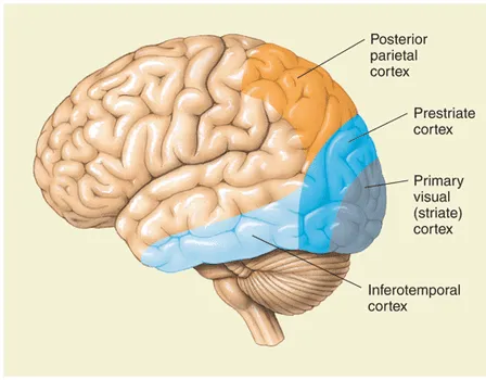
primary-visual.png — The visual cortex is located in the occipital lobe

primary visual cortex has 140 million neurons
two types of artificial neuron: perceptron, sigmoid neuron
perceptron takes binary inputs and produces a single binary output.
perceptrons should be considered as making decisions after weighing up evidence (inputs)
neural nets can express NAND, which means any computation can be built using these gates!

/projects/ml/dl/feedforward/ch1/
nand.svg

sigmoid neurons

you want to tweak the weights and biases such that small changes in either will produce a small change in the output
as such we must break free from the sgn step function and introduce the sigmoid function

/projects/ml/dl/feedforward/ch1/
sgn.svg — Binary, Discontinuous Sign

\(\leadsto\)

/projects/ml/dl/feedforward/ch1/
sig.svg — Continuous, Differentiable Sigmoid

thus the mathematics of \(\varphi\) becomes: \[\begin{align*} \sigma(z) &\equiv \cfrac{1}{1+e^{-z}}\\ &\implies \cfrac{1}{1+\text{exp}(-\sum_j w_jx_j -b)} \end{align*}\]