Multilayer Perceptron
We have seen what can be learned by the perceptron algorithm — namely, linear decision boundaries for binary classification problems.
It may also be of interest to know that the perceptron algorithm can also be used for regression with the simple modification of not applying an activation function (i.e. the sigmoid). I refer the interested reader to open another tab.
We begin with the punchline:
XOR
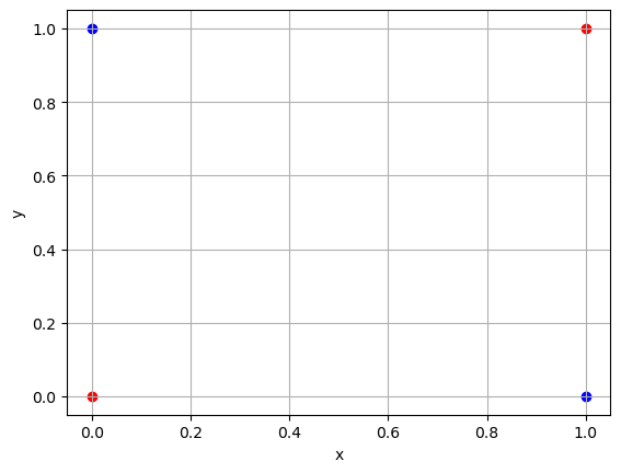
Now clearly, taking a ruler, your finger or positioning any straight-lined object on the above figure will not enable you to separate the blue (true) from the red (false) circles. This was also one of Marvin Minsky's arguments against further development of the Perceptron in 1963. However, with the benefit of hindsight, we shall not retire so quickly, instead we add another layer of the neurons:
Whilst this above architecture does not immediately solve our problem it puts us on the correct trajectory.
Propositional Logic
At some point we were going to have to deal with the logical interpretation of XOR.
XOR, denoted by the symbol \(\oplus\) means the logical exclusive or. Which translates colloquially to:
\(x_1\) or \(x_2\), but not both
We can express this sentiment in logical syntax
\[x_1 \oplus x_2 \equiv (x_1 \lor x_2) \land \neg (x_1 \land x_2)\]
and then construct smaller diagrams that express the \(\lor\), \(\land\) and \(\neg\land\).
Piecing these together (notice we now have weights), and taking the \(\land\) of these two:
To reproduce the mathematical equivalence we are looking for:\[x_1 \oplus x_2 \equiv (x_1 \lor x_2) \land \neg (x_1 \land x_2)\]
The overlapping \(x_1\)'s and \(x_2\)'s yield the glorious MLP:
Manual Trace
We now test all of our points to see if they are correctly classified by the above MLP:
-
[1,1]:- lights up the \(x_1\) and \(x_2\) nodes.
- the first pushes up +1 to \(h_1\) and -1 to \(h_2\)
- the bias is defeated at \(h_1\) and thus will now fire
- \(h_2\)'s bias causes it to fire by default, and the -1 charge from \(x_1\) maintains this
- next, we get the charges from \(x_2\): +1 to \(h_1\) and -1 to \(h_2\).
- the \(h_1\) becomes more positive, and thus certainly fires, whilst \(h_2\) has now been dragged below the 0 threshold.
- now, for the next layer to fire, since it is an
ANDneuron, you must have both \(h_1\) and \(h_2\) fired. - thus, y will not fire this time.
- Continuing with this line of thought, for [0,0] the MLP does not fire either. Only \(h_2\) does, and as we have seen a moment ago this is not sufficient.
- Fires! Do the trace to check.
- Also fires! Yay.
Linear Decision Boundary in Hidden State Space
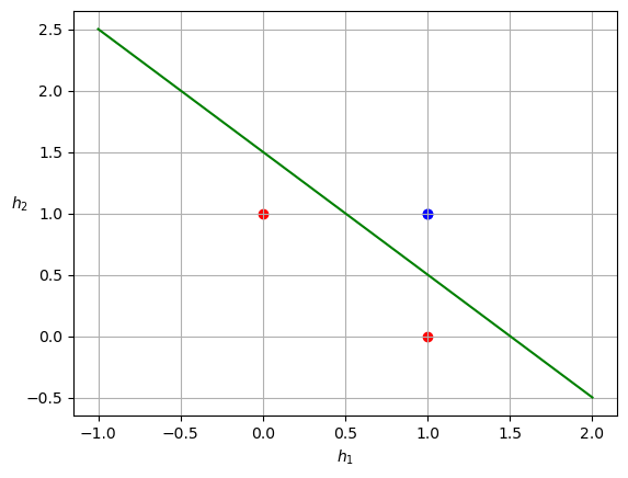
From the above trace we can summarise the following results:
| \(x_1\) | \(x_2\) | \(h_1\) | \(h_2\) |
| 1 | 1 | 1 | 0 |
| 0 | 0 | 0 | 1 |
| 1 | 0 | 1 | 1 |
| 0 | 1 | 1 | 1 |
And produce the a linear decision boundary in the \(h_1 / h_2 \) state space!
Original State Space
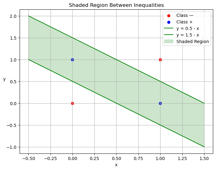
Reverting to our original state space, we can see that plotting the weights corresponds to using TWO linear inequality boundaries!
Truth Table (optional)
This part can be skipped but I do consider it of value to understand the problem that I am working on from all angles.
| \(x_1\) | \(x_2\) | \(\land\) | \(\lor\) | \(\neg\land\equiv\bar{\land}\equiv~\uparrow\) | \(\neg\lor\equiv\bar{\lor}\equiv~\downarrow\) | \(\oplus\) |
| 1 | 1 | 1 | 1 | 0 | 0 | 0 |
| 0 | 0 | 0 | 0 | 1 | 1 | 0 |
| 1 | 0 | 0 | 1 | 1 | 0 | 1 |
| 0 | 1 | 0 | 1 | 1 | 0 | 1 |
A benefit of this analysis is noticing that we have another equivalence for the XOR:
\[x_1 \oplus x_2 \equiv (x_1 \land x_2) \downarrow (x_1 \downarrow x_2), \text{where }\downarrow\text{ represents \texttt{NOR}}\]
A Single Neuron
Also, for reference, here is a single neuron:
The Problem with XOR
Now, as beautiful and rewarding this manual derivation is, it is not always possible to know how many neurons you will need to be able to linearly separate your data in a different state space.
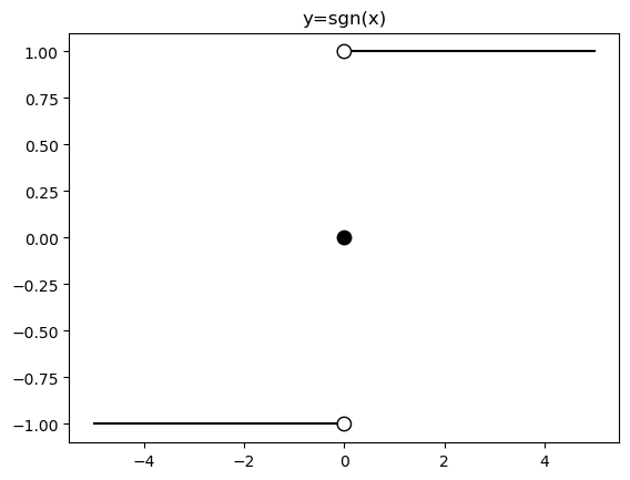
It is also worth acknowledging that we introduced a degree of non-linearity by using the step-function activation at the hidden nodes ⊕ — this function is not differentiable, and is now nearing the end of its shelf life. As such we must refactor the wheel:
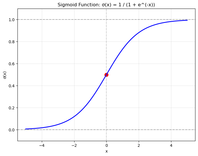
Real world problems – such as MNIST tackled in the last heading of this page – have hundreds of inputs with thousands of weights across tens of layers. ⊕
Backpropagation is the bridge between simple Perceptrons and Deep Learning with Multi-layered Perceptrons. We will now solve 3-XOR by Backpropagation.
\(N^2\)-XOR / Advanced XOR
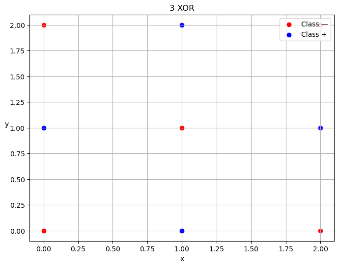
I call this problem \(N^2\) XOR. It makes sense to extend our XOR of two inputs ([0,1]), to that of three inputs ([0,1,2]).
In general we could extend the problem to any integer N, and the number of dots would be \(N^2\).
Code
Here we implement a MLP in Pytorch, train it using binary cross-entropy loss and visualise the hidden layer activations and outputs. We will also in a moment make use of the ability to set weights manually, but for now we will let the network use random initialisations of 0.15.
import torch
import torch.nn as nn
import matplotlib.pyplot as plt
import torch.utils.data
import torch.nn.functional as F
import pandas as pd
import numpy as np
import argparse


class MLP(torch.nn.Module):
    def __init__(self, hid=4, act='sig'):
        super(MLP, self).__init__()
        # two hidden layers
        self.act = act
        self.in_hid  = nn.Linear(2, hid)
        self.hid_out = nn.Linear(hid, 1)
        self.hid = None

    def forward(self, input):
        self.hid = torch.sigmoid(self.in_hid(input))
        if self.act == 'step':
            self.hid = (self.in_hid(input) >= 0).float()
            return (self.hid_out(self.hid) >= 0).float()
        else:         # sigmoid
            self.hid = torch.sigmoid(self.in_hid(input))
            return torch.sigmoid(self.hid_out(self.hid))

    def set_weights(self):
        in_hid_weight  = [[1.0,-1.0],[-1.0,1.0],[-1.0,-1.0],[1.0,1.0]]
        hid_bias       = [-0.5,-0.5,1.5,-2.5]
        hid_out_weight = [[1.0,1.0,1.0,1.0]]
        out_bias       = [-1.5]

        self.in_hid.weight.data = torch.tensor(
             in_hid_weight, dtype=torch.float32)
        self.in_hid.bias.data   = torch.tensor(
                hid_bias,   dtype=torch.float32)
        self.hid_out.weight.data= torch.tensor(
             hid_out_weight,dtype=torch.float32)
        self.hid_out.bias.data  = torch.tensor(
                 out_bias,  dtype=torch.float32)

def train(net, train_loader, optimizer):
    total=0
    correct=0
    for batch_id, (data,target) in enumerate(train_loader):
        optimizer.zero_grad()    # zero the gradients
        output = net(data)       # apply network
        loss = F.binary_cross_entropy(output,target)
        loss.backward()          # compute gradients
        optimizer.step()         # update weights
        pred = (output >= 0.5).float()
        correct += (pred == target).float().sum()
        total += target.size()[0]
        accuracy = 100*correct/total
    if epoch % 100 == 0:
        print('ep:%5d loss: %6.4f acc: %5.2f' %
             (epoch,loss.item(),accuracy))
    return accuracy

def test(net):
    with torch.no_grad(): # suppress updating of gradients
        net.eval()        # toggle batch norm, dropout
        correct=0
        total=0
        for batch_id, (data,target) in enumerate(train_loader):
            output = net(data)       # apply network
            loss = F.binary_cross_entropy(output,target)
            pred = (output >= 0.5).float()
            correct += (pred == target).float().sum()
            total += target.size()[0]
            accuracy = 100*correct/total
        net.train() # toggle batch norm, dropout back again
        return accuracy.item();

def graph_hidden(net, node):
    xrange = torch.arange(start=-0.5,end=2.5,step=0.01,dtype=torch.float32)
    yrange = torch.arange(start=-0.5,end=2.5,step=0.01,dtype=torch.float32)

    xcoord = xrange.repeat(yrange.size()[0])
    ycoord = torch.repeat_interleave(yrange, xrange.size()[0], dim=0)
    grid = torch.cat((xcoord.unsqueeze(1),ycoord.unsqueeze(1)),1)

    with torch.no_grad(): # suppress updating of gradients
        net.eval()        # toggle batch norm, dropout
        output = net(grid)
        net.train()
        hid = (net.hid >= 0.5).float()
        # plot function computed by model
        plt.clf()
        plt.pcolormesh(xrange,yrange,(hid.cpu()[:,node]).view(yrange.size()[0],xrange.size()[0]), cmap='Wistia', shading='auto')
        plt.xticks([0,1,2])
        plt.yticks([0,1,2])

def graph_output(net):
    xrange = torch.arange(start=-0.5,end=2.5,step=0.01,dtype=torch.float32)
    yrange = torch.arange(start=-0.5,end=2.5,step=0.01,dtype=torch.float32)
    xcoord = xrange.repeat(yrange.size()[0])
    ycoord = torch.repeat_interleave(yrange, xrange.size()[0], dim=0)
    grid = torch.cat((xcoord.unsqueeze(1),ycoord.unsqueeze(1)),1)

    with torch.no_grad(): # suppress updating of gradients
        net.eval()        # toggle batch norm, dropout
        output = net(grid)
        net.train()       # toggle batch norm, dropout back again
        pred = (output >= 0.5).float()
        # plot function computed by model
        plt.clf()
        plt.pcolormesh(xrange,yrange,pred.cpu().view(yrange.size()[0],xrange.size()[0]), cmap='Wistia')
        plt.xticks([0,1,2])
        plt.yticks([0,1,2])

 # command-line arguments
class Args:
    def __init__(self):
	self.hid = 5               # number of hidden units
	self.act = 'sig'           # activation function: 'sig' or 'step'
	self.init = 0.15           # initial weight size
	self.set_weights = False   # whether to set weights manually
	self.lr = 0.001            # learning rate
	self.epoch = 200000        # max training epochs

# Create an instance of Args with default values
args = Args()

df = pd.read_csv('check.csv')

data = torch.tensor(df.values,dtype=torch.float32)

num_input = data.shape[1] - 1

full_input  = data[:,0:num_input]
full_target = data[:,num_input:num_input+1]

# print(full_input)

train_dataset = torch.utils.data.TensorDataset(full_input,full_target)
train_loader  = torch.utils.data.DataLoader(train_dataset,
				 batch_size=train_dataset.__len__())

# choose network architecture
net = MLP(args.hid,args.act)

if list(net.parameters()):
    # initialize weight values
    if args.set_weights:
	net.set_weights()
    else:
	for m in list(net.parameters()):
	    m.data.normal_(0,args.init)

    # delete this
    graph_output(net)
    plt.scatter(full_input[:,0],full_input[:,1],
		c=full_target[:,0],cmap='brg_r',vmin=-2,vmax=1)
    #plt.savefig('./plot/check.jpg',format='jpg')
    plt.show()

    # use Adam optimizer
    optimizer = torch.optim.Adam(net.parameters(),lr=args.lr,
				 weight_decay=0.00001)
    #optimizer = torch.optim.SGD(net.parameters(),lr=args.lr,momentum=0.9,
    #                            weight_decay=0.00001)

    accuracy = 0
    if args.set_weights:
	print('Initial Weights:')
	for m in list(net.parameters()):
	    print(m.data)
	accuracy = test(net)
	print('Initial Accuracy: ',accuracy)

    # training loop
    if args.act == 'sig' and accuracy < 100.0:
	epoch = 0
	count = 0
	while epoch < args.epoch and count < 2000:
	    epoch = epoch+1
	    accuracy = train(net, train_loader, optimizer)
	    if accuracy == 100:
		count = count+1
	    else:
		count = 0
	print('Final Weights:')
	for m in list(net.parameters()):
	    print(m.data)
	accuracy = test(net)
	print('Final Accuracy: ',accuracy)

    # graph hidden units
    if args.hid <= 30:
	for node in range(args.hid):
	    graph_hidden(net, node)
	    plt.scatter(full_input[:,0],full_input[:,1],
			c=full_target[:,0],cmap='brg_r',vmin=-2,vmax=1)
	    #plt.savefig('./plot/hid_%d_%d.jpg' \                       % (args.hid, node))
	    plt.show()

    # graph output unit
    graph_output(net)
    plt.scatter(full_input[:,0],full_input[:,1],
		c=full_target[:,0],cmap='brg_r',vmin=-2,vmax=1)
    #plt.savefig('./plot/out_%d.jpg' %args.hid ,format='jpg')
    plt.show()
Results
5 nodes
Creating a neural network to learn the weights with 5 hidden nodes was possible. We can observe the output and understand where on our MLP architecture these weights sit:
tensor([[ 6.2529,  6.2611],
	[ 8.0631,  8.0715],
	[ 7.0275, -5.3862],
	[-1.5961, -1.6023],
	[ 5.8470, -7.3902]])
tensor([-24.1028, -11.7520,  10.9807,   2.3644, -10.9280])
tensor([[-13.6477, -12.2777,  12.0103, -20.0231,  -6.7899]])
tensor([4.4831])
Final Accuracy: 100.0The above figure was generated by ChatGPT.
Hidden Unit Dynamics
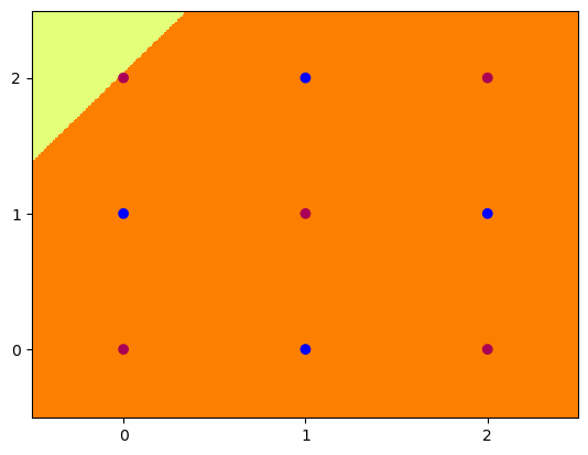
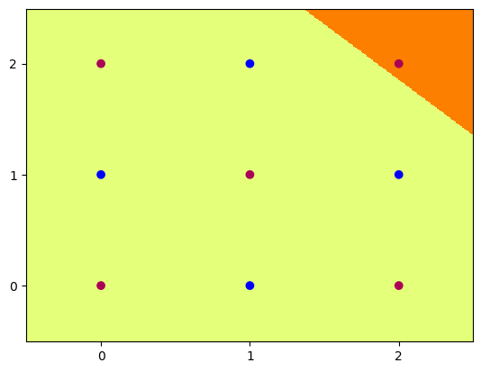
We can also visualise what each of these hidden nodes was responsible for contributing to the overall segmentation of blue dots from red:
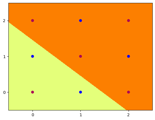
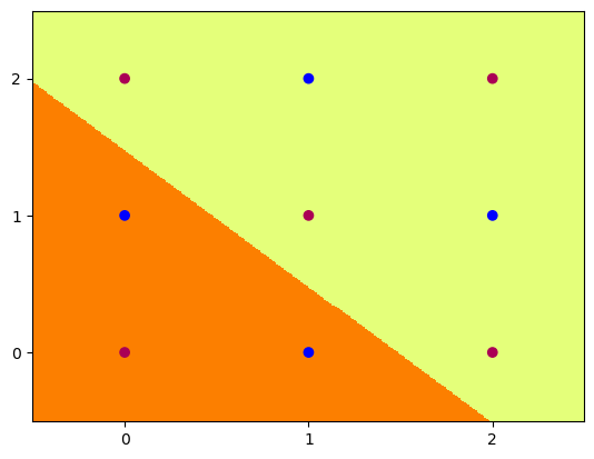
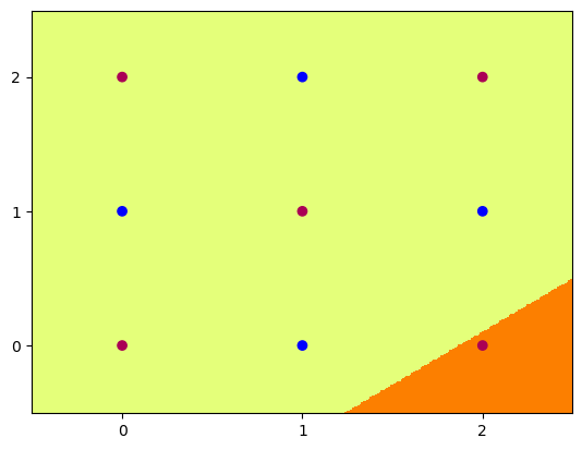
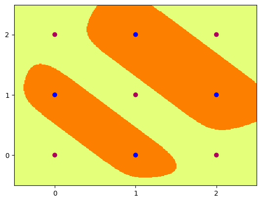
4 nodes
Trying to achieve the same effect with 4 nodes is a different story. Running the Code above for 200,000 epochs multiple times still does not allow it to converge to 100% accuracy, and thus the task is never learned. We can however input the initialisation weights manually after studying the problem on paper to produce:
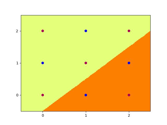
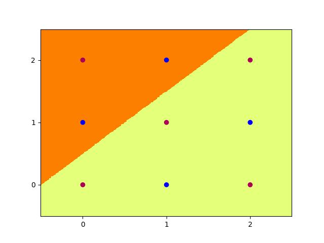
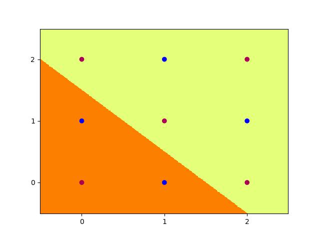
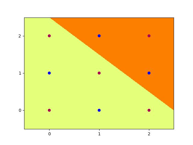
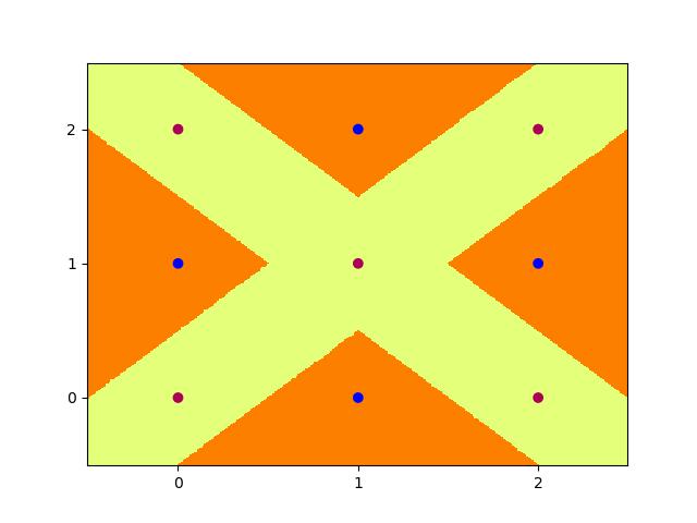
With weights
in_hid_weight  = [[1.0,-1.0],[-1.0,1.0],[-1.0,-1.0],[1.0,1.0]]
hid_bias       = [-0.5,-0.5,1.5,-2.5]
hid_out_weight = [[1.0,1.0,1.0,1.0]]
out_bias       = [-1.5]
Conclusion
In conclusion, we can see that MLP's are beautiful, and the logical next step in a world where perceptron learning works. Furthermore, we notice the fragility of the model to initial weights, and the way in which it is sometimes just unable to produce the correct global optima and instead sits in a local one. Finally, Machine Learning continues to be as much art as science in that we must sprinkle the right amounts of non-linearity in the right places to get our puppet to jiggle and dance.
I leave you with a small code snippet from geeksforgeeks who use the tensorflow library to leverage MLP's and a modern pipeline to classify the MNIST dataset.
Code
## Importing necessary modules
import tensorflow as tf
import numpy as np
import matplotlib.pyplot as plt
from tensorflow.keras.models import Sequential
from tensorflow.keras.layers import Flatten, Dense

# Load MNIST dataset
(x_train, y_train), (x_test, y_test) = tf.keras.datasets.mnist.load_data()

# Normalize image pixel values by dividing by 255 (grayscale)
gray_scale = 255

x_train = x_train.astype('float32') / gray_scale
x_test = x_test.astype('float32') / gray_scale

# Checking the shape of feature and target matrices
print("Feature matrix (x_train):", x_train.shape)
print("Target matrix (y_train):", y_train.shape)
print("Feature matrix (x_test):", x_test.shape)
print("Target matrix (y_test):", y_test.shape)

# Visualizing 100 images from the training data
fig, ax = plt.subplots(10, 10)
k = 0
for i in range(10):
    for j in range(10):
        ax[i][j].imshow(x_train[k].reshape(28, 28), aspect='auto')
        k += 1
plt.show()

# Building the Sequential neural network model
model = Sequential([
    # Flatten input from 28x28 images to 784 (28*28) vector
    Flatten(input_shape=(28, 28)),

    # Dense layer 1 (256 neurons)
    Dense(256, activation='sigmoid'),

    # Dense layer 2 (128 neurons)
    Dense(128, activation='sigmoid'),

    # Output layer (10 classes)
    Dense(10, activation='softmax'),
])

# Compiling the model
model.compile(optimizer='adam',
              loss='sparse_categorical_crossentropy',
              metrics=['accuracy'])

# Training the model with training data
model.fit(x_train, y_train, epochs=10,
          batch_size=2000,
          validation_split=0.2)

# Evaluating the model on test data
results = model.evaluate(x_test, y_test, verbose=0)
print('Test loss, Test accuracy:', results)
Results
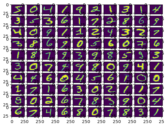
Test loss, Test accuracy: [0.27164116501808167, 0.92330002784729]