Predicting Life Expectancy
Intro
The focus here is on EDA (Exploratory Data Analysis) and investigating the best choice for the \(\lambda\) hyperparameter for LASSO and Ridge Regression.
We will be working on the Life Expectancy CSV data obtained from WHO.
Peeking at Data
We begin by viewing the columns of the Life Expectancy Dataframe:
  import seaborn as sns
  import pandas as pd
  import matplotlib.pyplot as plt

  pd.options.display.float_format = '{:.2f}'.format
  le_df = pd.read_csv("life_expectancy.csv")
  le_df.columns
Index(['Country', 'Year', 'Status', 'Life expectancy ', 'Adult Mortality',
       'infant deaths', 'Alcohol', 'percentage expenditure', 'Hepatitis B',
       'Measles ', ' BMI ', 'under-five deaths ', 'Polio', 'Total expenditure',
       'Diphtheria ', ' HIV/AIDS', 'GDP', 'Population',
       ' thinness  1-19 years', ' thinness 5-9 years',
       'Income composition of resources', 'Schooling'],
      dtype='object')
We can then view the range of our life expectancy values with a box plot:
sns.boxplot(x=le_df['Life expectancy '])
plt.show()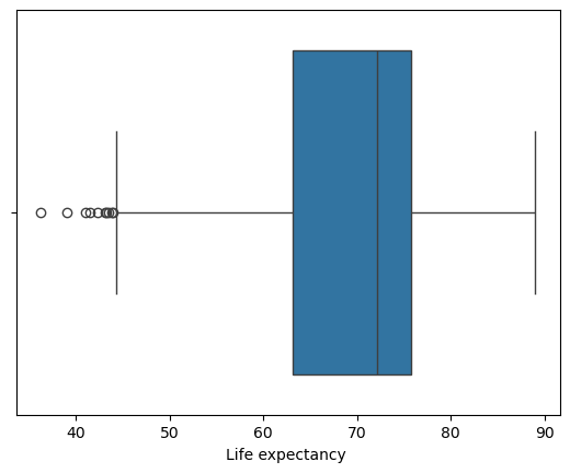
From here we can glean
- the folks that died early at late 30's, early 40's;
- the minimum and maximum excluding these outliers (whiskers)
- the first and third Quartiles; and
- the mean (\(\mu\)) life expectancy
le_df.info()<class 'pandas.core.frame.DataFrame'> RangeIndex: 2938 entries, 0 to 2937 Data columns (total 22 columns): # Column Non-Null Count Dtype --- ------ -------------- ----- 0 Country 2938 non-null object 1 Year 2938 non-null int64 2 Status 2938 non-null object 3 Life expectancy 2928 non-null float64 4 Adult Mortality 2928 non-null float64 5 infant deaths 2938 non-null int64 6 Alcohol 2744 non-null float64 7 percentage expenditure 2938 non-null float64 8 Hepatitis B 2385 non-null float64 9 Measles 2938 non-null int64 10 BMI 2904 non-null float64 11 under-five deaths 2938 non-null int64 12 Polio 2919 non-null float64 13 Total expenditure 2712 non-null float64 14 Diphtheria 2919 non-null float64 15 HIV/AIDS 2938 non-null float64 16 GDP 2490 non-null float64 17 Population 2286 non-null float64 18 thinness 1-19 years 2904 non-null float64 19 thinness 5-9 years 2904 non-null float64 20 Income composition of resources 2771 non-null float64 21 Schooling 2775 non-null float64 dtypes: float64(16), int64(4), object(2) memory usage: 505.1+ KB
Correlations
Then to produce a correlation matrix we would require exclusively continuous values. As such I have dropped those that are not:
le_df = le_df.drop(columns=['Country','Status']) import numpy as np
corr_mat = le_df.corr()
mask = np.zeros_like(corr_mat, dtype=bool)
mask[np.triu_indices_from(mask)] = True
f, ax = plt.subplots(figsize=(20,19))
cmap=sns.diverging_palette(220,10, as_cmap=True)
sns.heatmap(corr_mat, mask=mask, cmap=cmap, vmax=.3, center=0,
square=True, linewidths=.5, cbar_kws={"shrink": .5})
plt.show()Note: We only need to view the lower / upper triangular section of the matrix due to the symmetry.
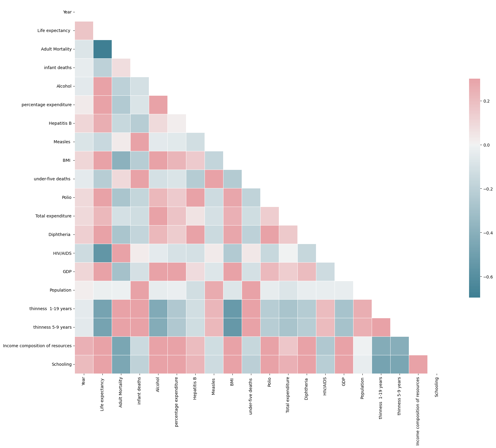
Letting our libraries continue doing the heavy lifting for us:
    sns.pairplot(le_df)
    plt.show()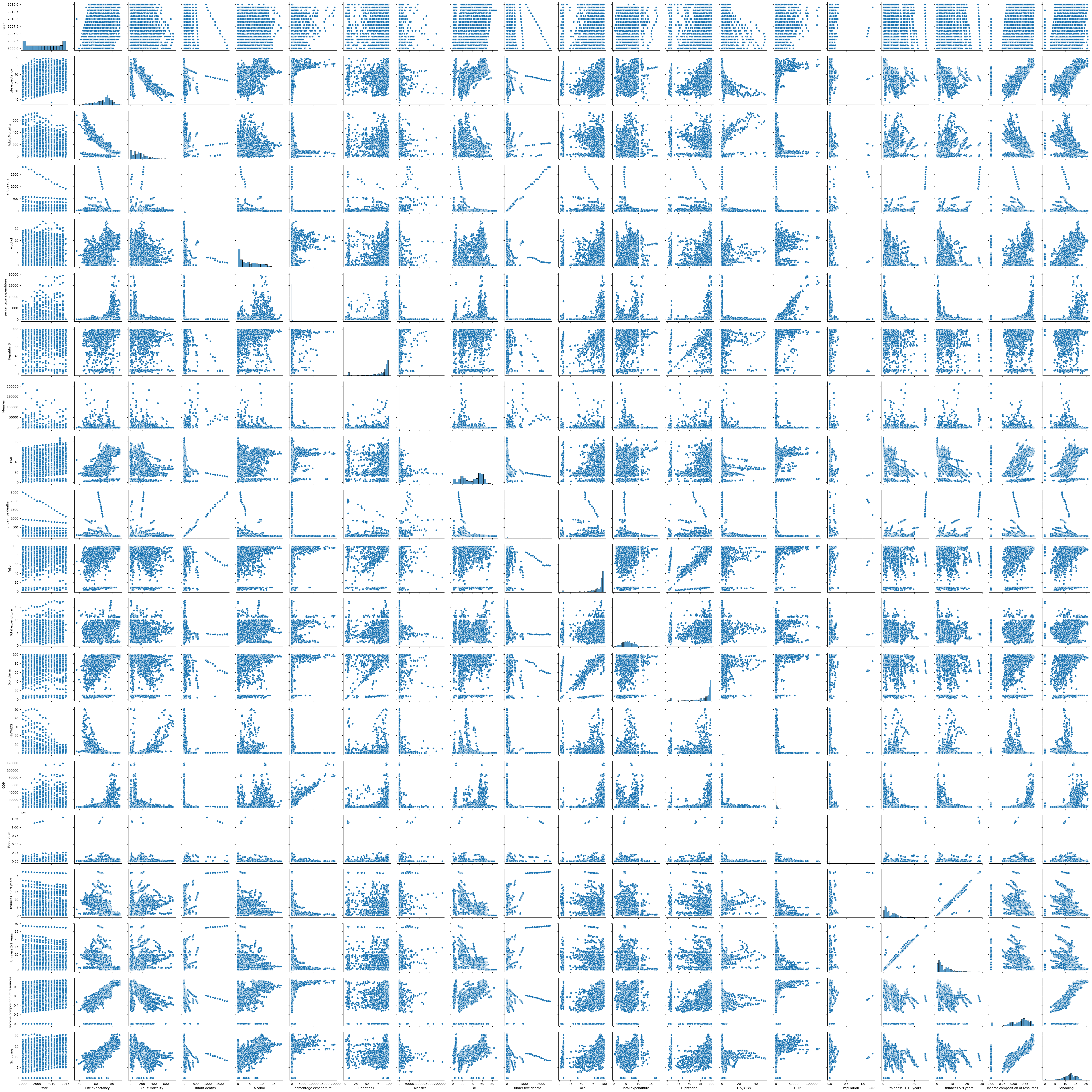
From here we learn that Adult Mortality is very negatively correlated with Life Expectancy (which makes sense). Also the 3 most positively correlated features with Life Expectancy are
- HIV/AIDS 0.753
- Income Comp of Resources 0.729
- Schooling 0.722
All of which are interesting in their own right.
Standard Scaling
Because we will be using regularised regression today and the penalties on weight will be affected by the magnitudes of the features we must first standardise our data:
  from sklearn.preprocessing import StandardScaler

  le_df_noNAN = le_df.dropna()
  X = le_df_noNAN.drop(columns=["Life expectancy "])
  y = le_df_noNAN["Life expectancy "].copy()

  scaler = StandardScaler().fit(X)
  scaled_X = scaler.transform(X)

  print(f"Feature Means: {scaled_X.mean(axis=0)}")
  print(f"Feature Variances: {scaled_X.var(axis=0)}")
Feature Means: [-7.96290464e-15 -7.75607595e-17 -4.30893108e-18 6.89428973e-17 2.58535865e-17 1.63739381e-16 -4.30893108e-18 -6.89428973e-17 -2.58535865e-17 2.57458632e-16 1.68048312e-16 1.29267933e-17 6.03250352e-17 8.61786217e-17 -3.01625176e-17 5.60161041e-17 -7.75607595e-17 1.72357243e-16 7.92843319e-16] Feature Variances: [1. 1. 1. 1. 1. 1. 1. 1. 1. 1. 1. 1. 1. 1. 1. 1. 1. 1. 1.]
Splitting Training and Test Data
Now we split the testing and training data
  from sklearn.model_selection import train_test_split
  X_train, X_test = train_test_split(X, test_size=0.2, random_state=73)
  y_train, y_test = train_test_split(y, test_size=0.2, random_state=73)
Empiricism on Lambda (Ridge)
And start training a Ridge regression with varying values of the hyperparameter lambda:
  %%time
  import warnings
  warnings.filterwarnings("ignore")
  from sklearn.linear_model import Ridge
  lambdas = [0.01, 0.1, 0.5, 1, 1.5, 2, 5, 10, 20, 30, 50, 100, 200, 300]
  N = len(lambdas)
  coefs_mat = np.zeros((X_train.shape[1], N))
  for i in range(N):
    L = lambdas[i]
    ridge_lm = Ridge(alpha=L).fit(X_train, y_train)
    coefs_mat[:,i] = ridge_lm.coef_

  plt.figure(figsize=(10,10))
  for i in range(X_train.shape[1]):
    lab = "X" + str(i + 1)
    plt.plot(np.log(lambdas), coefs_mat[i], label=lab)
    plt.legend()
  plt.xlabel(r"log($\lambda$)")
  plt.ylabel("Estimated Coefficient")
  plt.show()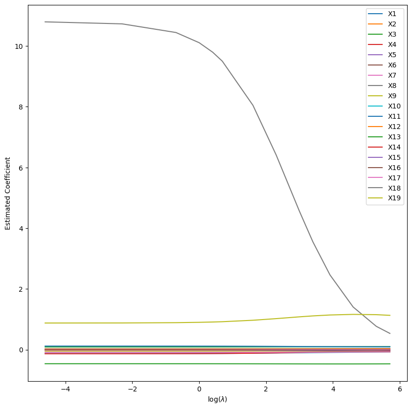
We then find the best Lambda:
  %%time
  lambdas = np.arange(0,50.1,step=0.1)
  n = X_train.shape[0]
  N = lambdas.shape[0]
  CV_score = np.zeros(N)
  curIdx = 0
  #X_train = X_train.to_numpy()
  #y_train = y_train.to_numpy()
  for L in lambdas:
    sq_errs = 0.
    for i in range(100):
      x_i = X_train[i]
      x_removed_i = np.delete(X_train, i, axis=0)
      y_i = y_train[i]
      y_removed_i = np.delete(y_train, i, axis=0)

      mod = Ridge(alpha=L).fit(x_removed_i, y_removed_i)
      sq_errs += (mod.predict(x_i.reshape(1,-1))-y_i)**2

    CV_score[curIdx] = sq_errs/n
    curIdx += 1

  min_idx = np.argmin(CV_score)
  plt.plot(lambdas, CV_score)
  plt.xlabel(r"log($\lambda$)")
  plt.ylabel("LOOCV (Ridge)")
  plt.axvline(x=lambdas[min_idx], color='red')
  plt.annotate(f"$\lambda = {lambdas[min_idx]}$", xy=(25,1800))
  plt.show()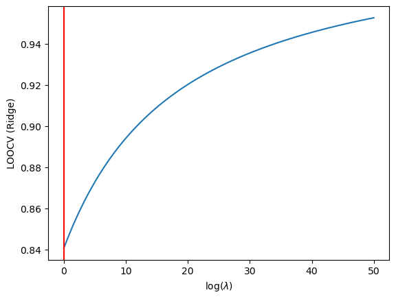
Empiricism on Lambda (LASSO)
We then repeat for our L1 regularisation model:
  from sklearn.linear_model import Lasso
  lambdas = [0.01, 0.1, 0.5, 1, 1.5, 2, 5, 10, 20, 30, 50, 100, 200, 300]
  N = len(lambdas)
  coefs_mat = np.zeros((X_train.shape[1], N))
  for i in range(N):
    L = lambdas[i]
    ridge_lm = Lasso(alpha=L).fit(X_train, y_train)
    coefs_mat[:,i] = ridge_lm.coef_

  plt.figure(figsize=(10,10))
  for i in range(X_train.shape[1]):
    lab = "X" + str(i + 1)
    plt.plot(np.log(lambdas), coefs_mat[i], label=lab)
    plt.legend()
  plt.xlabel(r"log($\lambda$)")
  plt.ylabel("Estimated Coefficient")
  plt.show()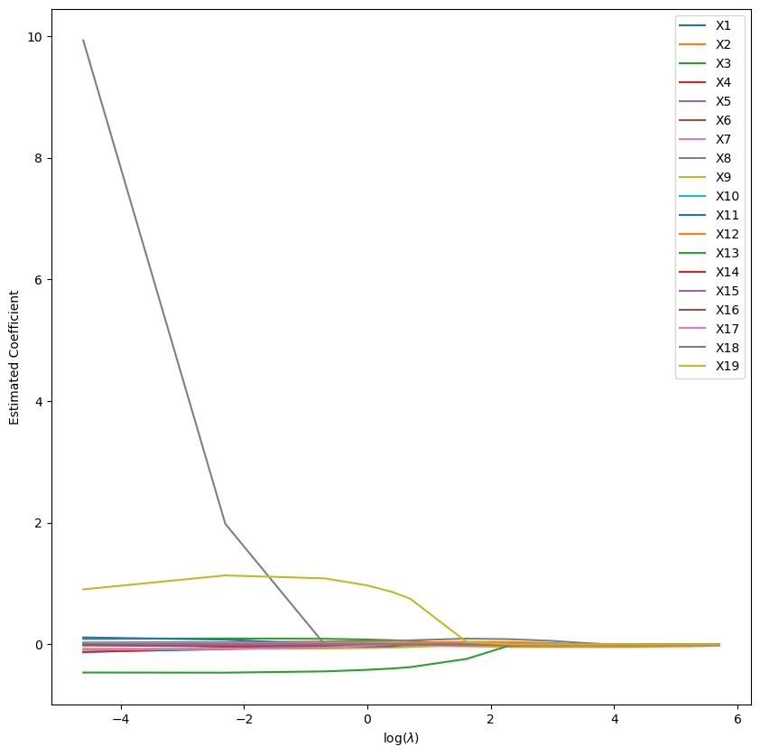
Thus we find the optimal lambda to be…
  %%time
  lambdas = np.arange(0,50.1,step=0.1)
  n = X_train.shape[0]
  N = lambdas.shape[0]
  CV_score = np.zeros(N)
  curIdx = 0
  #X_train = X_train.to_numpy()
  #y_train = y_train.to_numpy()
  for L in lambdas:
    sq_errs = 0.
    for i in range(20): #note we are not going to N
      x_i = X_train[i]
      x_removed_i = np.delete(X_train, i, axis=0)
      y_i = y_train[i]
      y_removed_i = np.delete(y_train, i, axis=0)

      mod = Lasso(alpha=L).fit(x_removed_i, y_removed_i)
      sq_errs += (mod.predict(x_i.reshape(1,-1))-y_i)**2

    CV_score[curIdx] = sq_errs/n
    curIdx += 1

  min_idx = np.argmin(CV_score)
  plt.plot(lambdas, CV_score)
  plt.xlabel(r"log($\lambda$)")
  plt.ylabel("LOOCV (Lasso)")
  plt.axvline(x=lambdas[min_idx], color='red')
  plt.annotate(f"$\lambda = {lambdas[min_idx]}$", xy=(25,1800))
  plt.show()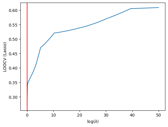
Results
It seems that in both situations we have fucked up. The LASSO and Ridge hyperparameters are being found to be 0. A quick fitting of the traning data to sklearn's LassoCV model may help clear some confusion:
  from sklearn.linear_model import LassoCV
  from sklearn.metrics import mean_squared_error
  m_lassoCV = LassoCV(cv=5).fit(X_train, y_train)
  ypred_train_lassoCV = m_lassoCV.predict(X_train)
  ypred_test_lassoCV = m_lassoCV.predict(X_test)
  print(f"Mean Squared Error (TRAIN): {mean_squared_error(y_train,ypred_train_lassoCV)}")
  print(f"Mean Squared Error (TEST) : {mean_squared_error(y_test, ypred_test_lassoCV)}")
  print(f"With Lambda as {m_lassoCV.get_params()}")
Mean Squared Error (TRAIN): 62.824553484016874
Mean Squared Error (TEST) : 68.37568737602082
With Lambda as {'alphas': None, 'copy_X': True, 'cv': 5, 'eps': 0.001, 'fit_intercept': True, 'max_iter': 1000, 'n_alphas': 100, 'n_jobs': None, 'positive': False, 'precompute': 'auto', 'random_state': None, 'selection': 'cyclic', 'tol': 0.0001, 'verbose': False}
Conclusion
The above shows that our analysis was not incorrect in attempting to determine the most optimal \(\lambda\)s, but rather a mistake has occurred in the preprocessing step causing the statistical signifance of my data to become muddled. In a later refactoring I may come back and improve my preprocessing, or abandon it completely in favour of a more homogenous dataset.
  from sklearn.metrics import r2_score
  print(f'Train Accuracy: {r2_score(ypred_train_lassoCV, y_train)}')
  print(f'Test Accuracy: {r2_score(ypred_test_lassoCV, y_test)}')
Train Accuracy: -8.965044425866656 Test Accuracy: -7.17445447809699